Travel Map

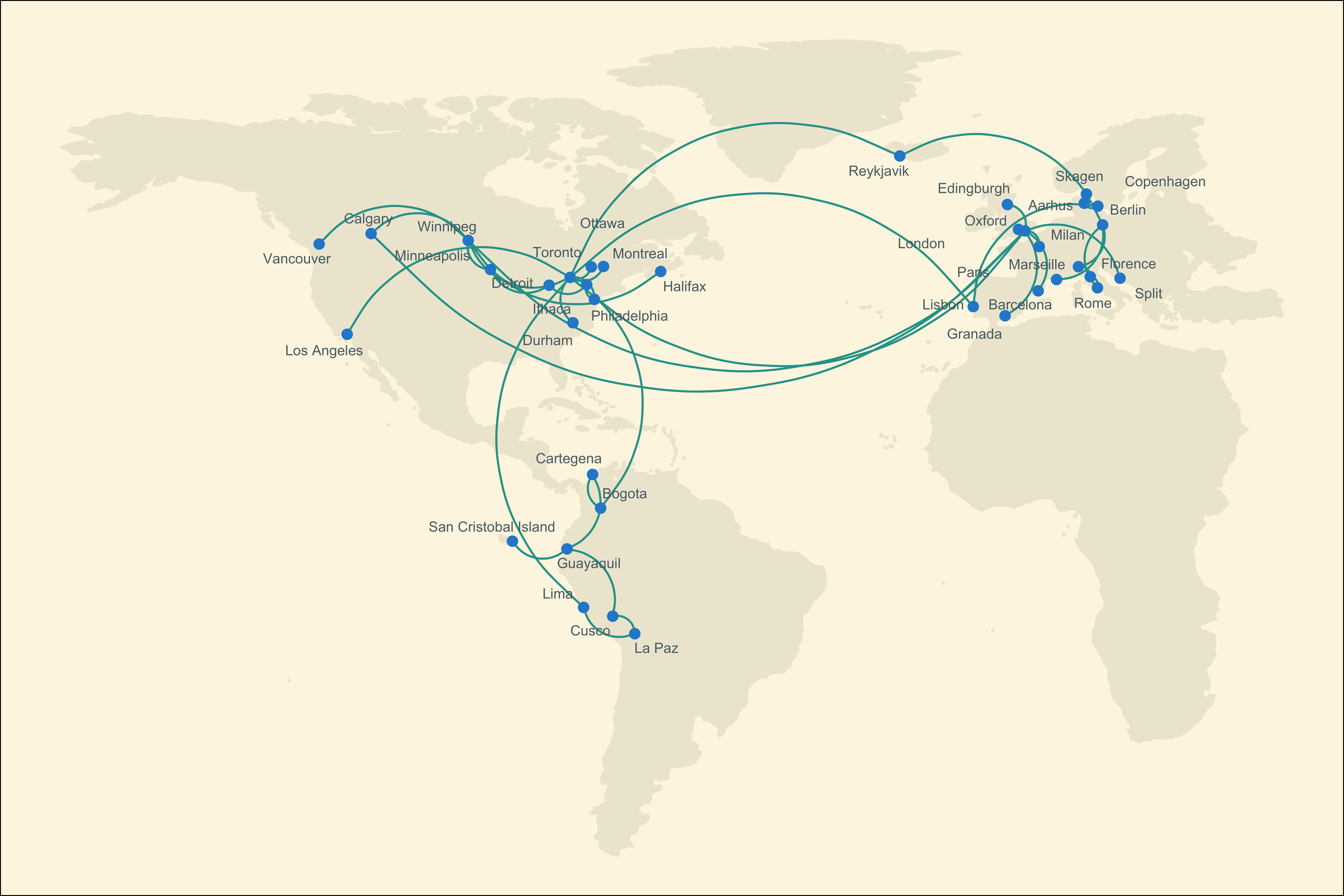
I want to see as much of the world as possible while I can. The map I’m making here will serve as a reminder of the memories I made around the world, and as motivation to go out and see the rest.

I’ve made the map in Rmarkdown so anyone reading who has a basic familiarity with R and Rstudio should be able to easily make their own.

To make the map I used R, ggplot, and Google’s geolocation API. I relied heavily on The Lucid Manager’s post in which he creates his own.

First loading all the necessary libraries

suppressPackageStartupMessages({
  library(tidyverse)
  library(ggmap)
  library(ggrepel)
  library(maps)
  library(here)
})

Here I’m setting internal filepaths. To reproduce the code below, replace the here() functions with the urls in the comments.

path_flights <- here("static", "map", "trips.csv")
#path_flights <- "https://raw.githubusercontent.com/aridf/travel-map/master/data/trips.csv"
path_geos <- here("static", "map", "geos.csv")
#path_geos <- "https://raw.githubusercontent.com/aridf/travel-map/master/data/geos.csv"

Loading the data. I had to add country info to some of the cities to ensure the google API searches for the correct city. I remove this later so it does not show up in my visualization.

flights <- read_csv(path_flights)
head(flights)

## # A tibble: 6 x 2
##   From       To         
##   <chr>      <chr>      
## 1 Bogota     Cartegena  
## 2 Cartegena  Guayaquil  
## 3 Cusco      La Paz     
## 4 Detroit    Minneapolis
## 5 Durham     Toronto    
## 6 Edingburgh London

Here I’m deleting duplicates and return flights. This helps reduce the clutter in the visual.

d <- vector()
for (i in 1:nrow(flights)) {
    d <- which(paste(flights$From, flights$To) 
               %in% paste(flights$To[i], flights$From[i]))
    flights$From[d] <- "R"
}
flights <- flights %>%
  filter(From != "R") %>%
  select(From, To)

Next, I grab coordinate data from the google API. I use two layers of conditions to limit the number of calls I’m making to the API. First, I check if I already have a list of locations and coordinates saved. If not, I get a list of all the locations in my flight list and call that API for each. If I already have some coordinates saved, I just check to see if there are any new locations. If there are, I call the API for the new entries only. If not, then I move ahead with my previous dataset.

locations <- unique(c(flights$From, flights$To))
if(file.exists(path_geos)) {
  geos <- read_csv(path_geos)
  new <- locations[!(locations %in% geos$airport)]
  if(length(new) > 0) {
    geos <- new %>%
      geocode() %>%
      mutate(airport = new) %>%
      bind_rows(geos) %>%
      select(airport, lon, lat)
    write_csv(geos, path_geos)
  }
} else {
  new <- unique(c(flights$From, flights$To))
  geos <- new %>%
    geocode() %>%
    mutate(airport = new) %>%
    select(airport, lon, lat)
  write_csv(geos, path_geos)
}
head(geos)

## # A tibble: 6 x 3
##   airport       lon    lat
##   <chr>       <dbl>  <dbl>
## 1 Skagen      10.6   57.7 
## 2 Lisbon      -9.14  38.7 
## 3 Copenhagen  12.6   55.7 
## 4 Aarhus      10.2   56.2 
## 5 La Paz     -68.1  -16.5 
## 6 Bogota     -74.1    4.71

Merging trip data and coordinates.

flights <- merge(flights, geos, by.x = "To", by.y = "airport")
flights <- merge(flights, geos, by.x = "From", by.y = "airport")
head(flights)

##        From        To      lon.x     lat.x      lon.y     lat.y
## 1    Aarhus    Skagen  10.579186 57.725004   10.20392 56.162939
## 2    Berlin Marseille   5.369780 43.296482   13.40495 52.520007
## 3    Berlin     Milan   9.189982 45.464204   13.40495 52.520007
## 4    Bogota Cartegena -75.479426 10.391049  -74.07209  4.710989
## 5   Calgary  Winnipeg -97.138374 49.895136 -114.07085 51.048615
## 6 Cartegena Guayaquil -79.922359 -2.170998  -75.47943 10.391049

Removing country info from the city names here.

geos$airport <- geos$airport %>%
  word(1, sep = ",")

Creating my world map object. I’m setting the size limits of my map dynamically. This enables the map to expand dynamically as I travel to more regions of the world

#set size limits of the worldmap. Prevent unvisited regions from displaying
xmin <- min(geos$lon) - 10
xmax <- max(geos$lon) + 10
ymin <- min(geos$lat) - 10
ymax <- max(geos$lat) + 10

#get map
worldmap <- borders("world", xlim = c(xmin, xmax), ylim = c(ymin, ymax), 
                    colour = "#eee8d5", fill = "#eee8d5")

This is the actual plot. The layers are pretty straightforward:

geom_curve creates curved lines connecting “From” and “To”.
geom_point adds dots at each location
geom_text_repel add labels while giving them room to breathe

ggplot() + worldmap + 
    geom_curve(data = flights, aes(x = lon.x, y = lat.x, xend = lon.y, 
                                   yend = lat.y), col = "#2aa198", size = .4) + 
    geom_point(data = geos, aes(x = lon, y = lat), col = "#268bd2") + 
    geom_text_repel(data = geos, color = "#586e75", aes(x = lon, y = lat, label = airport), 
               col = "black", size = 2, segment.color = NA, segment.size = 1) + 
    theme_void() +
    theme(panel.background = element_rect(fill = "#fdf6e3"))

Finally, save out the file to a folder on my website so I can read it in as an image elsewhere.

ggsave(
  filename = here("static", "map", "travel_map.png"),
  width = 7.5,
  height = 4.5,
  units = "in",
  dpi = 300
)